Design Basic Concepts
Basic Concepts
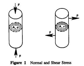
Stress is force per unit area, F/A. Typical units of stress are MPa, and N/mm2. Although there are many names given to stress, there are only two primary types, differing in the orientation of the loaded area. With normal stress, σ, the area is normal to the force carried. With shear stress, τ, the area is parallel to the force.
Strain, ε, is elongation expressed on a fractional or percentage basis. It may be listed as having units of mm/mm, and percent, or no units at all. A strain in one direction will be accompanied by strains in orthogonal directions in accordance with Poisson’s ratio, (εy, νεx, νεz).
Hooke’s Law
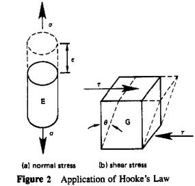
Hooke’s law is a simple mathematical statement of the relationship between elastic stress and strain; stress is proportional to strain. For normal stress, the constant of proportionality is the modulus of elasticity (Young’s Modulus), E.
σ = Eε
For shear stress, the constant of proportionality is the shear modulus, G.
τ = Gθ
Elastic Deformation
Since stress is F/A and strain δ/Lo, Hooke’s law can be expanded in form to give the elongation of an axially loaded member experiencing normal stress.
Tension loading is considered to be positive; compression loading is negative.
![]()
The actual length of a member under loading is given by:
L = Lo ± δ
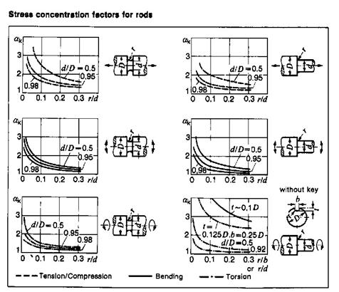
Stress Concentrations
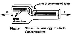
Stress concentrations occur whenever there is a discontinuity or non-uniformity in an object. Examples of non-uniform shapes are lapped shafts, plates with holes and notches, and shafts with keyways. It is convenient to think of stress as streamlines within an object. There will be a stress concentration wherever local geometry forces the streamlines closer together.
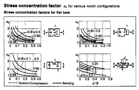
Stress values determined by simplistic F/A, Mc/I, or Tr/J calculation will be greatly understated. Stress concentration factors (stress risers) are correction factors used to account for the non-uniform stress distributions. The symbol k is often used, but this not universal. The actual stress is determined as the product of the stress concentration factor, k, and the ideal stress. Values of stress concentration factor are almost always greater then 1.0, and can run as 3.0 and above. The exact value for a given application must be determined from extensive experimentation or from published tabulations or charts of standard configurations.
σ' = k σ
|
Approximate Stress Concentration Factors |
|
|
Bending or direct tension |
|
|
Concentric groove around cylindrical shaft |
|
|
Ration of groove radius to shaft diameter |
Stress concentration factor |
|
r/d |
k |
|
0.1 |
2.0 |
|
0.5 |
1.6 |
|
1.0 |
1.2 |
|
2.0 |
1.1 |
|
Fillet |
|
|
Ratio of fillet radius to depth of member |
Stress concentration factor |
|
r/d |
k |
|
0 (sharp corner) |
2 |
|
1/16 |
1.75 |
|
1/8 |
1.5 |
|
1/4 |
1.2 |
|
1/2 |
1.1 |
|
Torsion |
|
|
Fillet in cylindrical shaft |
|
|
Ratio of fillet radius to radius of smaller shaft |
Stress concentration factor |
|
r/r |
k |
|
0.02 |
1.8 |
|
0.10 |
1.2 |
|
0.20 |
1.1 |
Combined Stresses
Loading is rarely confined to a single direction. Many practical cases have different normal and shear stresses on two or more perpendicular planes. Sometimes, one of the stresses may be small enough to be disregarded, reducing the analysis to one dimension. In most cases, however, the shear and normal stresses must be combined to determine the maximum stress acting on the material.
For any point in a loaded specimen, a plane can be found where the shear stress is zero. The normal stresses associated with this plane are known as the principal stresses, which are the maximum and minimum acting at that point in any direction.
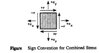
Proper sign convention must be adhered to when using the combined stress equations. As is usually the case, tensile normal stresses are positive; compressive normal stresses are negative. In two dimensions, shear stresses are designated as clockwise (positive) or counter clockwise (negative).
The maximum and minimum values of normal stress are the principal stresses.
![]()
The extreme shear stresses (i.e., maximum and minimum shear stress).
![]()
Dynamic Loading
If the load is applied to a structure suddenly, the structure’s response will be composed of two parts; a transient response (which decay to zero) and steady-state response. (These two parts are also known as the dynamic and static responses.)
Arbitrary multiplicative factors are applied to the steady-state stress to determine the maximum transient; a dynamic factor of 2.0 might be used.
Alternating Stress
Many parts are subject to a combination of static and reversed loading. Failure cannot be determined solely by comparing stresses with yield strength or endurance limit. The combined effects of the average stress and amplitude of the reversal must be considered. This is done graphically on a diagram that plots the mean stress versus the alternating stresses.
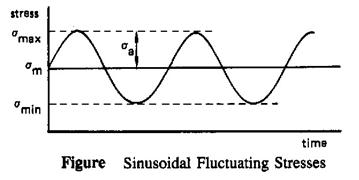
The mean stress is
![]()
The alternating stress is half of the range stress.
![]()
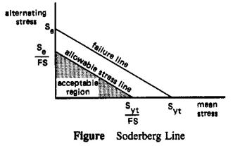
A criterion for acceptable design (or for failure) is established by graphically relating the yield strength and the endurance limit. One method of relating this information is a Soderberg line. From the figure, if the point (σm, σa) falls below the allowable line, the design is acceptable.
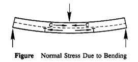
Bending Stress in Beams
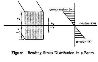
Normal stress occurs in a bending beam. Although it is a normal stress, the term bending stress or flexural stress is used to indicate the source of the of the stress. The lower surface of the beam experience tensile stress (which causes lengthening). The upper surface of the beam experiences compressive stress (which causes shortening). There is no stress along a horizontal plane passing through the centroid of the cross section, a plane known as the neutral plane or the natural axis.
Bending stress varies with location (depth) within the beam. It is zero at the neutral axis, and increases linearly with distance from the neutral axis, as predicted by the equation:
![]()
The bending moment, M, is used the equation. Ic is the centroid moment of inertia of the beam’s cross section. The negative sign, required by the convention that compression is negative, is commonly omitted.
Since the maximum stress will govern the design, y can be set equal to c to obtain extreme fiber stress. c is the distance from the neutral axis to the extreme fiber (i.e. the top or bottom most distant from the neutral axis).
![]()
The above equation shows that the maxim bending stress will occur where the moment is maximum. The region immediately adjacent to the point of maximum bending moment is called the dangerous section of the beam. The dangerous section can be found from a bending moment or shear diagram.
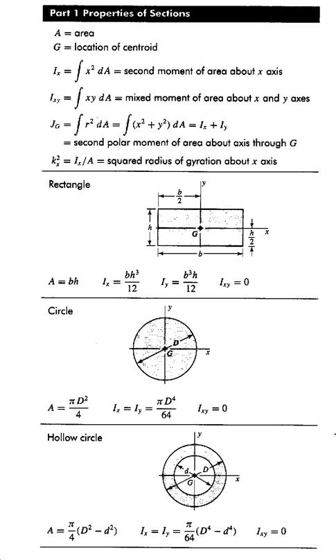
The moment of inertia, I, (it is the beam ability to resist bending).
Ic Moment of inertia (of plane areas) the sum of the products of all cross sectional elements by the squares of their distance from the neutral axis.
Shaft Design (Torsion – Twisting)
Shear stress occurs when shaft is placed in torsion. The shear stress at the outer surface of a bar or radius r, which is torsionally loaded by a torque T, is
![]()
J is the shaft’s polar moment of inertia. For a solid round shaft,
![]()
For a hollow round shaft,
![]()
If a shaft of length L carries a torque T, the angle of twist (in radians) will be
![]()
G is the shear modulus (8.0 x 10⁴ MPa). The shear modulus also can be calculated from the modulus of elasticity.
![]()
The polar moment of inertia, J (measure of an area’s resistance to torsion (twisting).
J = Ix + Iy
Shear and Bending Moment Diagram
The value of shear and moment, V and M, will depend on location along the beam. It is much more convenient to describe the shear and moment function graphically. Graphs of shear and moment as function of position along the beam are known as shear and moment diagram. Drawing these diagrams does not require knowing the shape or area of the beam.
Poisson’s ratio
Experiments demonstrate that when a material is placed in tension, there exists not only an axial strain, but also a lateral strain. Passion demonstrated that these two strains were proportional to each other within the range of Hooke’s law. This constant is expressed as

and is known as Poisson’s ratio. These same relations apply for compression, except that a lateral expansion takes place instead.
The three elastic constants are related to each other as follows:
![]()
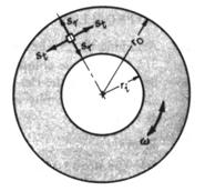
Stress in rotating disks
a) Solid disk:
![]()
b) Disk with hole:

where
σr max = maximum radial stress, N/m2
(» 400 N/mm2 for steel, 200 N/mm2 for cast iron)
σt max = maximum tangential stress, N/m2
(» 400 N/mm2 for steel, 200 N/mm2 for cast iron)
ρ = density, kg/m3 (7770 kg/m3 for steel, 7000 kg/m3 for cast iron)
ν = Poisson’s ratio (0.30 for steel, 0.27 for cast iron)
ri = inside diameter of plate, m
ro = outside diameter of plate, m
v = peripheral velocity, ro ω = 2 π ro (N/60), m/s (rotation speed, rpm).
For pressure plate made from cast iron, the centrifugal speed limited by the centrifugal force strength should not exceed 65-70 m/s